library(rClustering)
library(cluster)
library(glue)
library(dplyr)
library(tidyselect)
library(tidyr)
library(stringr)
library(ggplot2)
library(gridExtra)
library(kableExtra)
Synthetic clusters
Build the clusters
clusts <- make_clusters(4, c_range = c(-20, 20), density = 500, categorical = F, seed = 1)
clusts %>%
  sample_n(10) %>%
  kable() %>%
kable_material(c("striped", "hover"), full_width = F)| y_true | x | y |
|---|---|---|
| 1 | -11.621969 | -3.158619 |
| 1 | -8.281378 | -6.979358 |
| 3 | -12.552332 | 16.030500 |
| 1 | -10.828491 | -3.680739 |
| 1 | -9.308444 | -2.092698 |
| 3 | -11.584022 | 14.231961 |
| 1 | -10.087508 | -8.408464 |
| 1 | -7.257910 | -3.745361 |
| 3 | -10.429119 | 16.351010 |
| 4 | 16.405530 | 6.801611 |
Extract the cluster dimensions
clust_positions <- clusts %>%
  group_by(y_true) %>%
  summarize_all(list(min = min, max = max, mean = mean)) %>%
  select(sort(peek_vars()))

clust_plot_data <- clust_positions %>%
  pivot_longer(cols = !y_true) %>%
  mutate(coord = if_else(str_detect(name, "^y_"), "y", "x")) %>%
  mutate(name = str_sub(name, start = 3)) %>%
  pivot_wider(names_from = coord, values_from = value) %>%
  mutate(center = factor(name == "mean"))

clust_plot_data %>%
  head() %>%
  kable() %>%
kable_material(c("striped", "hover"), full_width = F)| y_true | name | x | y | center |
|---|---|---|---|---|
| 1 | max | -5.920596 | -1.602418 | FALSE |
| 1 | mean | -9.489214 | -5.077230 | TRUE |
| 1 | min | -12.569354 | -8.564183 | FALSE |
| 2 | max | 4.049007 | 17.464265 | FALSE |
| 2 | mean | 2.848125 | 16.245504 | TRUE |
| 2 | min | 1.727480 | 15.115688 | FALSE |
Plot the cluster dimensions and the cluster values
shapes <- c(16, 3)
names(shapes) <- c(F, T)
sizes <- c(3, 10)
names(sizes) <- c(F, T)

p1 <- clust_plot_data %>%
  ggplot(aes(x = x, y = y, col = y_true, shape = center, size = center)) +
  geom_point() +
  ggtitle("Cluster Dimensions") +
  coord_cartesian(xlim = c(-20, 20), ylim = c(-20, 20)) +
  scale_shape_manual(values = shapes) +
  scale_size_manual(values = sizes) +
  theme(legend.position = "none")

p2 <- clusts %>% ggplot(aes(x = x, y = y, col = y_true)) +
  geom_point() +
  ggtitle("Cluster Points") +
  coord_cartesian(xlim = c(-20, 20), ylim = c(-20, 20)) +
  theme(legend.position = "none")

grid.arrange(p1, p2, ncol = 2)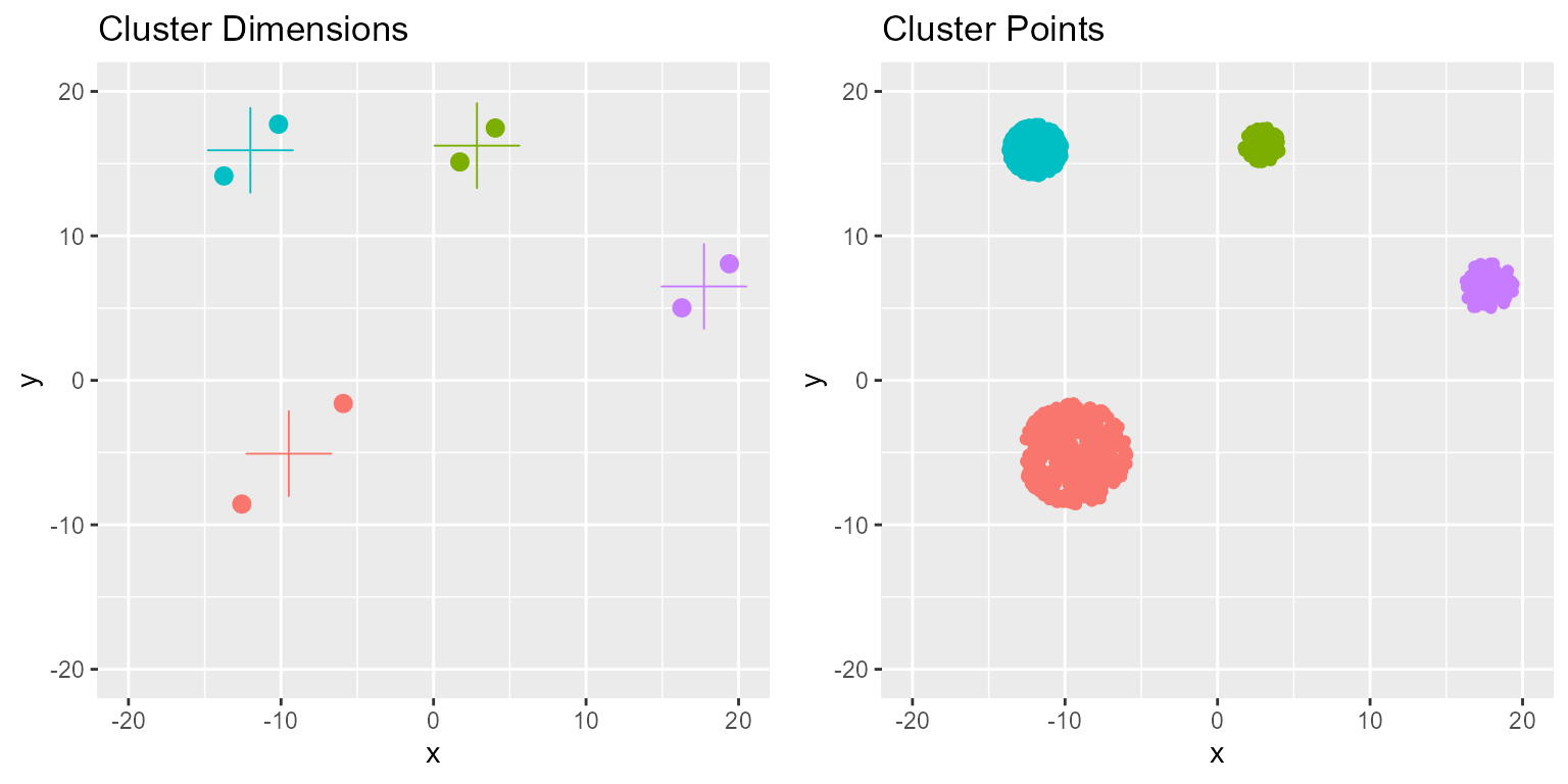
Since the clusters are perfect circles we can extract the center by taking the mean and the edges by taking the min and max of the coordinates.
Kmeans
Fit Kmeans
# Prepare clusters
clusts <- make_clusters(4, c_range = c(-20, 20), density = 500, categorical = F, seed = 2)

# Prepare arguments
vals <- setNames(data.frame(expand.grid(c(5, 10, 20), c(1, 10, 20))), c("n_iter", "n_start"))
vals$n_clust <- 4
vals$fit_name <- rep(c("A", "B", "C"), 3)

# Loop over argument combinations and fit Kmeans
out <- mapply(get_mean_clusters,
  fit_name = vals$fit_name,
  n_clust = vals$n_clust,
  iter = vals$n_iter,
  n_start = vals$n_start,
  MoreArgs = list(data = clusts, seed = 1),
  SIMPLIFY = F
) %>%
  bind_rows() %>%
  mutate(y_pred = factor(y_pred))
Visualize fits
p1 <- ggplot(out, aes(x = x, y = y, col = y_true)) +
  geom_point(size = 0.5) +
  ggtitle("Ground Truth") +
  theme(legend.position = "none")

p2 <- ggplot(out, aes(x = x, y = y, col = y_pred)) +
  geom_point(size = 0.5) +
  facet_wrap(~title, labeller = labeller(title = label_wrap_gen(20)), ncol = 3) +
  ggtitle("Kmeans", subtitle = "Varying Iterations and Starts") +
  theme(legend.position = "none")

grid.arrange(p1, p2,
  widths = c(3, 4), heights = c(3, 9),
  layout_matrix = rbind(
    c(1, NA),
    c(3, 3)
  )
)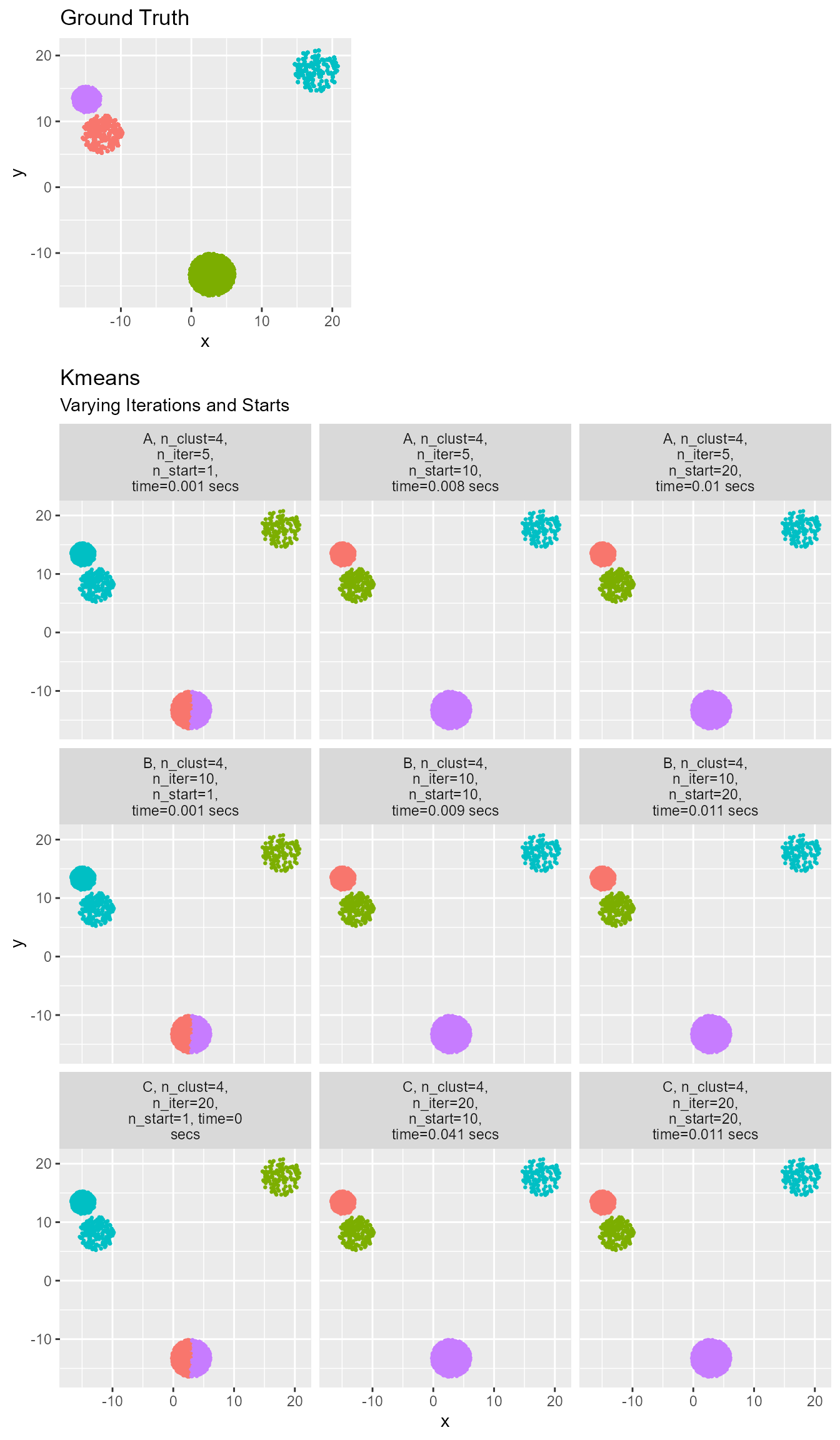
Note how important it is to use multiple starts so the model can converge. No amount of iterations will help if the starting point is very poor. Additionally, Kmeans is an unsupervised learning method. This means that it can find distinct clusters, but the clusters are not guaranteed to have the same label as the ground truth. The more iterations and starts specified the longer the fit takes.
Kprototypes
Fit Kprototypes
# Prepare clusters
clusts <- make_clusters(4, c_range = c(-20, 20), density = 500, categorical = 0.9, seed = 2)

# Prepare arguments
vals <- setNames(data.frame(expand.grid(c(5, 10, 20), c(1, 10, 20))), c("n_iter", "n_start"))
vals$n_clust <- 4
vals$fit_name <- rep(c("A", "B", "C"), 3)

# Loop over argument combinations and fit Kprototypes
out <- mapply(get_mean_clusters,
  fit_name = vals$fit_name,
  n_clust = vals$n_clust,
  iter = vals$n_iter,
  n_start = vals$n_start,
  MoreArgs = list(data = clusts, seed = 1),
  SIMPLIFY = F
) %>%
  bind_rows() %>%
  mutate(y_pred = factor(y_pred))
Visualize fits
p1 <- ggplot(out, aes(x = x, y = y, col = y_true)) +
  geom_point(size = 0.5) +
  ggtitle("Ground Truth") +
  theme(legend.position = "none")

p2 <- ggplot(out, aes(x = x, y = y, col = y_pred)) +
  geom_point(size = 0.5) +
  facet_wrap(~title, labeller = labeller(title = label_wrap_gen(20)), ncol = 3) +
  ggtitle("Kprototypes", subtitle = "Varying Iterations and Starts") +
  theme(legend.position = "none")

grid.arrange(p1, p2,
  widths = c(3, 4), heights = c(3, 9),
  layout_matrix = rbind(
    c(1, NA),
    c(3, 3)
  )
)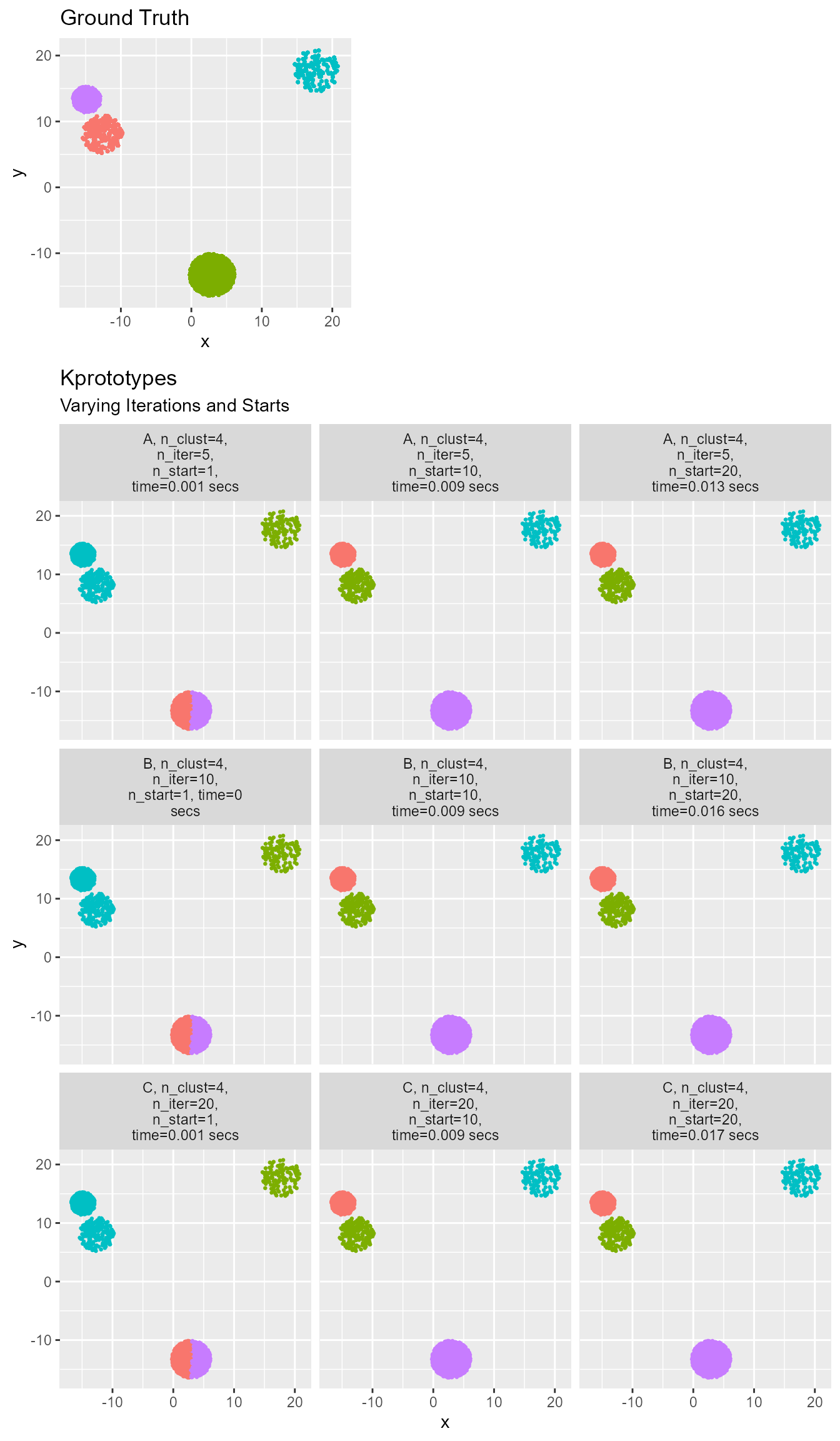
Note that the Kprototypes algorithm can handle the addition of a categorical variable that would be meaningless to Kmeans. Varying the start locations is still very important to finding a good solution.
Assessing cluster performance
# Basic Kmeans function
my_km <- function(data, k, seed){
  set.seed(seed)
  kmeans(x=data, centers=k, nstart=5, iter.max=100)
}

# Generate 4 cluster solution
n_clust <- 4
clusts <- make_clusters(n_clust, c_range = c(-20, 20), density = 500, categorical = F, seed = 3)

# Scale data for clustering
km_data <- clusts %>% select(x, y) %>% mutate_all(~scale(.) %>% as.vector())

# Look over [2, 8] clusters
ks <- seq(2, 8)

# Apply Kmeans to data for 2-8 clusters
fits <- lapply(ks, my_km, data=km_data, seed=1)
Sum of squares error elbow plot
# Extract SSE from fits
sses <- sapply(fits, function(x) x$tot.withinss)
sse_data <- data.frame(K=ks, SSE=sses)

p1 <- ggplot(clusts, aes(x = x, y = y, col = y_true)) +
  geom_point(size = 0.5) +
  ggtitle("Ground Truth") +
  theme(legend.position = "none")

p2 <- ggplot(sse_data, aes(x=K, y=SSE)) +
  geom_line() + geom_label(aes(label=scales::comma(SSE)), size=3) +
  scale_x_continuous(breaks=ks) + coord_cartesian(xlim=c(1, 10)) +
  scale_y_continuous(breaks=scales::pretty_breaks(n=8), labels=scales::comma_format()) +
  ggtitle("Sum of Squares Error for Different K", subtitle=glue("Ground truth: K={n_clust}"))

grid.arrange(p1, p2, ncol = 2)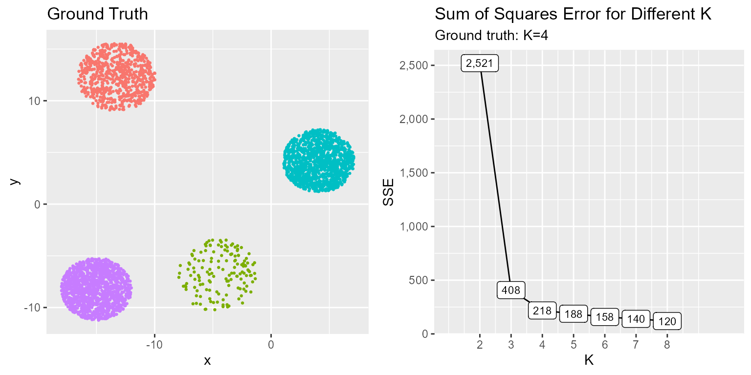
The SSE elbow plot illustrates the point at which adding more cluster centers no longer adds much value. A lower SSE is better, however, as K goes to infinity the SSE will generally decrease because we are adding additional centers. There is a point at which the decrease begins to stabilize, this is a good point to set K. In this case that point is K=4 as we see the curve flatten out thereafter. Additionally, the ground truth is that there are distinct clusters since we synthetically generated this data.
Silhouette index
# get distance of points from centers
euclidean_dist_mat <- daisy(km_data, metric="euclidean")

# get cluster labels from cluster solutions
clust_labs <- setNames(lapply(fits, function(x) x$cluster), glue("cluster_{ks}"))

# extract silhouette scores from cluster solutions
sil_summaries <- lapply(clust_labs, function(x, ...) summary(silhouette(x, ...)),
                        dist=euclidean_dist_mat)

# use average width as silhouette metric
sil_data <- data.frame(K=ks, avg.sil=sapply(sil_summaries, function(x) x$avg.width))
p1 <- ggplot(clusts, aes(x = x, y = y, col = y_true)) +
  geom_point(size = 0.5) +
  ggtitle("Ground Truth") +
  theme(legend.position = "none")

p2 <- ggplot(sil_data, aes(x=K, y=avg.sil)) +
  geom_line() + geom_label(aes(label=round(avg.sil, 2)), size=3) +
  scale_x_continuous(breaks=ks) +
  scale_y_continuous(name="Average Width", breaks=seq(0,1,0.2), labels=seq(0,1,0.2)) +
  coord_cartesian(xlim=c(1,10), ylim=c(0,1)) +
  ggtitle("Silhouette Average Width for Different K",  subtitle=glue("Ground truth: K={n_clust}"))

grid.arrange(p1, p2, ncol = 2)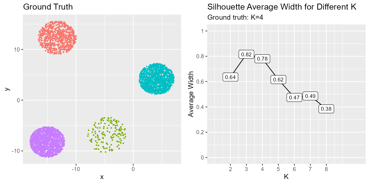
The silhoutte index ranges [-1, 1] where -1 indicates cluster label misalignment and 1 indicates perfect separation. In our case the optimal solution has K=4. However, from the results it would appear the optimal solution is K=3. Cluster performance assessment is part art and part science given the nature of unsupervised learning. What we determine the optimal solution to be from the data may not always be the ground truth but it should be close!